Super-Resolution

Article by James Zjalic (Verden Forensics) and Henk-Jan Lamfers (Foclar).

Problem

Events captured within video imagery utilised as evidence in trials are often at a distance from the camera lens, and thus, the resolution of the region is low. Although the resolution can be increased via rescaling using methods discussed in a previous blog post [1], doing so can increase the visibility of the individual pixels within the said region, leading to a coarse representation of such. Once block edges become visible, the human visionary system will treat them as discrete parts of an image, rather than the continuous manner that they are perceived when not visible.

Cause

Although the resolution of CCTV systems has gradually improved over time, it is still extremely common for video recordings to serve as exhibits that utilise low resolutions, either due to the use of an older system or the nonintentional conversion of a recording through a messaging application such as WhatsApp. Even in the best-case scenario, when the system used utilises a high resolution, the resolution of the region of interest within the imagery can be low due to the distance of such from the camera lens. When a low-resolution system is used to capture the imagery, the effects of distance are further compounded.

Solutions

The best solution to the problem would be to travel back in time prior to the event of interest and ensure there is a high-resolution CCTV system close to the event with the lens pointing directly at it. As time travel isn’t yet possible, the only option we have is to work with the imagery that has been captured and use a method to increase the resolution of the region of interest. Techniques that fall under this descriptor are called ‘Super-Resolution’, and these methods can provide higher resolution images in which the previously discussed blocking artefacts associated with nearest neighbour rescaling are less visible.

There are two distinct groups of super-resolution. The first is hallucination-based and can be referred to under different guises (e.g. single image super-resolution). This method employs a training step to learn the relationship between low-resolution and high-resolution captures of the same environment, followed by the application of this relationship to new images to predict missing high-resolution information. Deep learning is perfectly suited for the implementation of this technique, and the results can be good, but the method is not suitable for forensics due to the data prediction element, which can lead to changes to the data within an image that an examiner may not be aware of, and thus lead to inaccurate conclusions.

The second method is reconstruction-based or multiple image techniques. These use multiple frames of the same scene and utilise the differences between them to reconstruct detail. These differences can be geometric, such as differences in the position and distance of a camera lens to the object of interest, or photometric, such as differences in the lighting conditions [2].

The general approach consists of three steps [3], as follows.

First, Registration. This process determines the relationship between frames through alignment and the mapping of corresponding points to a single image. Once complete, all will share the same coordinate system.

Second, Interpolation. The images are interpolated through resampling to transform the set of coordinate locations into a high-resolution grid.

Third, de-blurring. High-frequency information that has been reduced during the previous stage is restored [4].

IMPLEMENTATION

The super-resolution filter [5] in Impress can be used on sequences with a moving object of interest (for example, a number plate). The plate should not be stationary, but if the object is moving too fast, the region would likely be subject to motion blur, which complicates matters. In Figure 1 the low resolution frames of a short video clip are shown. Below the sequence, the relative displacements of the LR-frames are shown. Only the sub-pixel displacements are plotted (range [-0.5,0.5] for both horizontal and vertical displacements). To the right of the plot, the high resolution SR image is displayed.

Figure 1: Sequence of low-resolution plates with sub-pixel shifts [-0.5,0.5] and resulting super-resolution image.

The (sub-)pixel displacements of the LR-frames are calculated in the registration step of the super-resolution filter. To start this phase, the operator has to select the first relevant frame of the short sequence the filter is applied to. This can be done by selecting a time range using the in and outpoint using the timeline control. After setting these points, the user must navigate back to the inpoint and add the super resolution filter to the pipeline (see Figure 2) and select a region of interest (ROI) containing the object of interest. The filter parameters can then be adjusted and the video replayed to the outpoint (or end of the video). The scale parameter determines the super-resolution scale factor and is maximised to 3.0 (300%). A simple of thumb is that when fewer images are available, a smaller scale factor is used, and when more images are available, a larger scale factor is best. For super-resolution to be effective, a minimum of four images should be used.

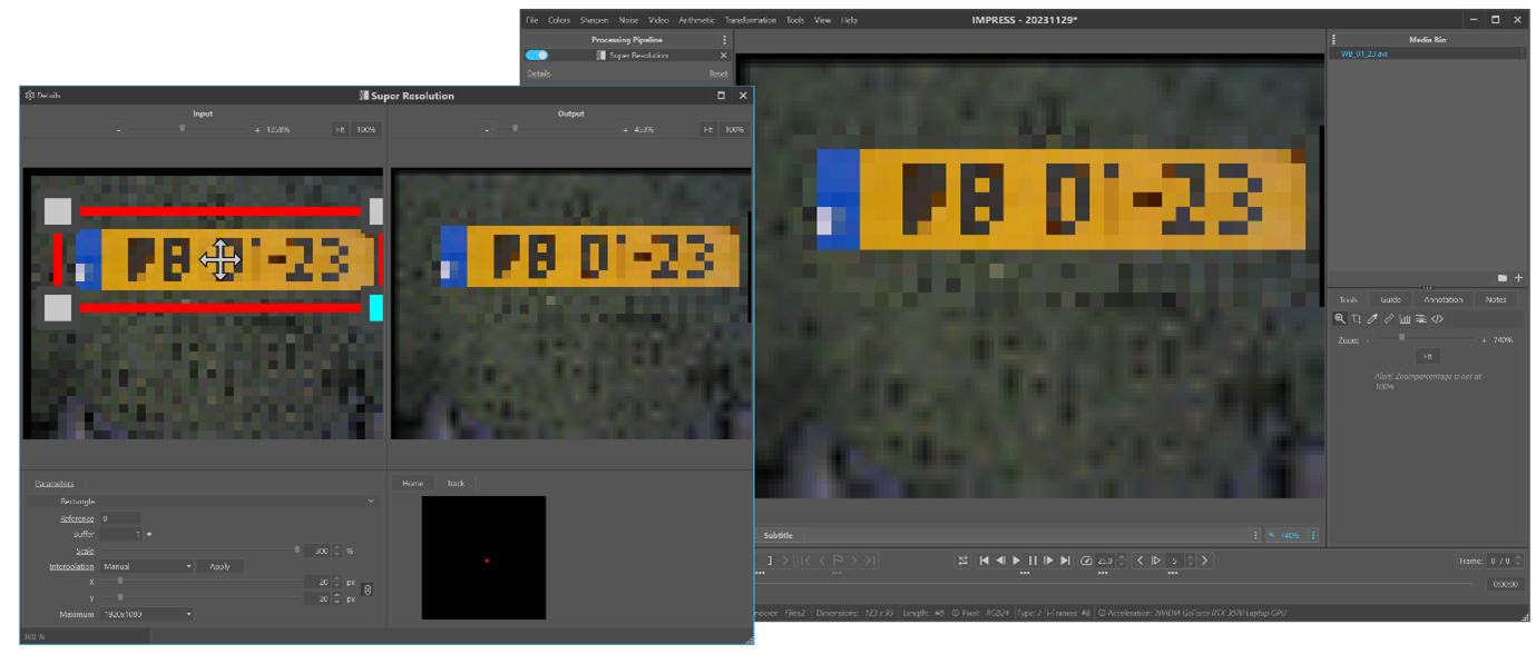
Figure 2: Loading the sequence in Impress and adjusting the parameters of the super resolution filter on the first frame.

After the registration of the relative sub-pixel displacements of the LR-frames, these frames are combined (frame fusion) into a high-resolution image. The fusion algorithm consists of two stages: weighted median interpolation followed by iterative weighted linear-interpolation using the result of the first stage as an input (first estimate). The LR-frames of pixel dimensions (W,H) are fused into one high-resolution image that has pixel dimensions: (S x W, S x H). The fusion step is only applied to the pixels in the original region of interest. The area of the SR-image outside the ROI are calculated by applying replicated scaling with scale factor S.

The processing can be accelerated by choosing the value manual for the interpolation parameter. In this case, only the median interpolation (stage 1) is used for the fusion step (see Figure 3). When reaching the end of the video (or outpoint) by pressing the ‘Apply’ button, the second stage (iterative weighted linear-interpolation) is calculated for the total collection of all frames in the selected time frame (see Figure 4).

Figure 3: Weighted Median interpolation super resolution result.

Figure 4: Iterative Weighted interpolation result.

The last (optional) step of the super-resolution process is the de-blur filtering. Due to errors in the sub-pixel displacements from the registration process the SR-image is blurred. The variations in the registration errors can be approximated by a Gaussian distribution, and the blur can be reduced by applying the general de-blur filter [6-7] on the SR-image. Although the plate was already clearly readable in Figure 4, one can observe the increase of sharpness in the de-blurred image of Figure 5. In less favourable cases, the de-blur step of the process can bring critical improvements to the end result.

Figure 5: Post-processing with a general deblur filter.

The whole process can be repeated with the same or other parameter values by navigating back to the in-point. The filter result is cleared and recalculated as the sequence is played again until the end (outpoint). Only by taking a snapshot is the SR-image (and/or de-blur image) saved to an image file.

Conclusion

Super-resolution is a technique that may assist when the resolution of a region of interest results in a coarse representation of such when rescaling using the nearest neighbour algorithm. However, considerations should be made as to whether it is suitable based on the method employed and the end user of the enhanced imagery. In order to make this judgement, an understanding of the method, including the interpolation algorithm, is essential to ensure that the end result does not add information to the image that is not present in the original version.

REFERENCES

[1]          Foclar and Verden Forensics, “Re-Scaling.” Accessed: Nov. 22, 2023. [Online]. Available: https://foclar.com/news/re-scaling

[2]          J. Satiro, K. Nasrollahi, P. L. Correia, and T. B. Moeslund, “Super-resolution of facial images in forensics scenarios,” in IEEE 5th International Conference on Image Processing Theory, Tools and Applications, 2015.

[3]          A. N. A. Rahim, S. N. Yaakob, R. Ngadiran, and M. W. Nasruddin, “An analysis of interpolation methods for super resolution images,” IEEE Stud. Conf. Res. Dev., 2015.

[4]          S. Villena, “Image super-resolution for outdoor digital forensics. Usability and legal aspects,” Comput. Ind., 2018.

[5]   R. Szeliski (2011) Computer Vision, Algorithms and Applications, p436 Springer.

[6]   Sonka M. Hlavac V. Boyle R. (2013) Image Processing, Analysis and Machine Vision, p164 Brooks/Cole Publishing Company.

[7]   Alan C. Bovik (2010) Handbook of Image and Video Processing, p173 Academic Press.

De-Haze

Article by James Zjalic (Verden Forensics) and Henk-Jan Lamfers (Foclar).

Problem

The most pronounced impact of haze on digital imagery is poor contrast, but it can also change the representation of colours within the environment and cause a reduction in the overall visibility of objects within [1]. Although generally not as problematic as other quality issues, image operations which follow are optimised if it is first addressed. In daytime captures it generally presents itself across entire frames as the distance of the sun from the illuminated environment is so vast that the lighting is consistent. During hours of darkness, the localised nature of artificial light can lead to haze effecting only specific regions within the frames.

Cause

Haze is defined as the suspension in the air of extremely small, dry particles which are invisible to the naked eye and sufficiently numerous to give the air an opalescent appearance [2]. The composition of these particles can vary - dust, water droplets, pollution from factories, exhaust fumes from vehicles and smoke or a mixture [3]. These particles mix with those in the atmosphere, absorbing light particles and scattering them in a manner not observed under normal conditions. The result is a suppression of the dynamic range of colours within a digital image relative to that when the haze is not present [4]. As the root cause is the interaction of light within the environment, it is added during the initial acquisition stage and is never added during transmission. Due to the physical nature of particles, its impact is generally across the entire length of a video rather than a few frames of a small region (notwithstanding recordings of a duration that would mean the suspended particles have dispersed from the capture environment or those in which the camera lens moves away from the suspended particles). Its impact becomes more evident the further from the camera lens the objects are as there are more suspended particles for the light particles to interact with between the object and the camera lens.

Solutions

Solutions to reduce haze within forensic imagery are not as heavily researched as those for other imagery operations such as brightening and sharpening, likely owing to the frequency in which it presents itself as a problem. Whilst the vast majority of imagery encountered within imagery forensics could benefit from some brightness and sharpening, the presence, and thus the requirement to reduce haze, is less common. It also differs from traditional enhancement techniques as the degradation is dependent on both the distance of objects and regional density of the haze.

With that being said, the issues haze causes in other sectors of imagery (such as video-guided transportation, surveillance and satellite) means a number of solutions have been proposed. The method can go by various names such as de-fogging, haze removal or de-haze, but all are used to define the operation of reducing the impact of haze on digital imagery.

One of the most simplistic methods is similar to that used in frame averaging, in which the random variation in the haze between frames is exploited, but this is only possible for video recordings (as multiple frames are required to obtain an average) and is not possible for imagery in which the lens is moving.

A second solution is histogram equalisation, a technique that distributes the range of grey tone pixels across a higher dynamic range, thus addressing the narrow range of grey and the reduction in contrast caused by haze. This method can be applied globally or locally, with the local method providing better quality results as it can accommodate varying depths of field. A halo effect can also occur when global adjustments are made as it cannot adapt to local regions of brightness [5]. 

The blackbody theory takes advantage of the expectation that objects which are known to be black should be represented by pixel values close to zero. Any drift from this value can then be attenuated. This theory assumes the atmosphere is homogenous and that the non-zero black object offset is constant. It would, therefore, not be applicable during hours of darkness or captures over distances that cause local haze effects [6].

Splitting an image into local blocks and maximising contrast to each block [7], utilising machine learning to understand the light and transmission maps (providing that other imagery under normal conditions of the scene is available) and frequency domain filtering [8] are amongst other methods proposed [9].

IMPLEMENTATION

In Impress, the dehaze filter [10] can reduce the effects of mist, smog, and sand storms on images and video frames. Depending on th degree of overexposure, the filter can also have positive effects when trying to suppress halos surrounding lights in the dark. When applying the filter, the atmospheric color has to be selected. The filter detail window (see Figure 1) has a colour picker control, which allows the user to select the colour by clicking on the Pick (pipet) and subsequently in an area of the left image (input image of the filter) which corresponds to the sky. With a click, the values of Red, Green and Blue are set to the values of the pixel that was clicked.

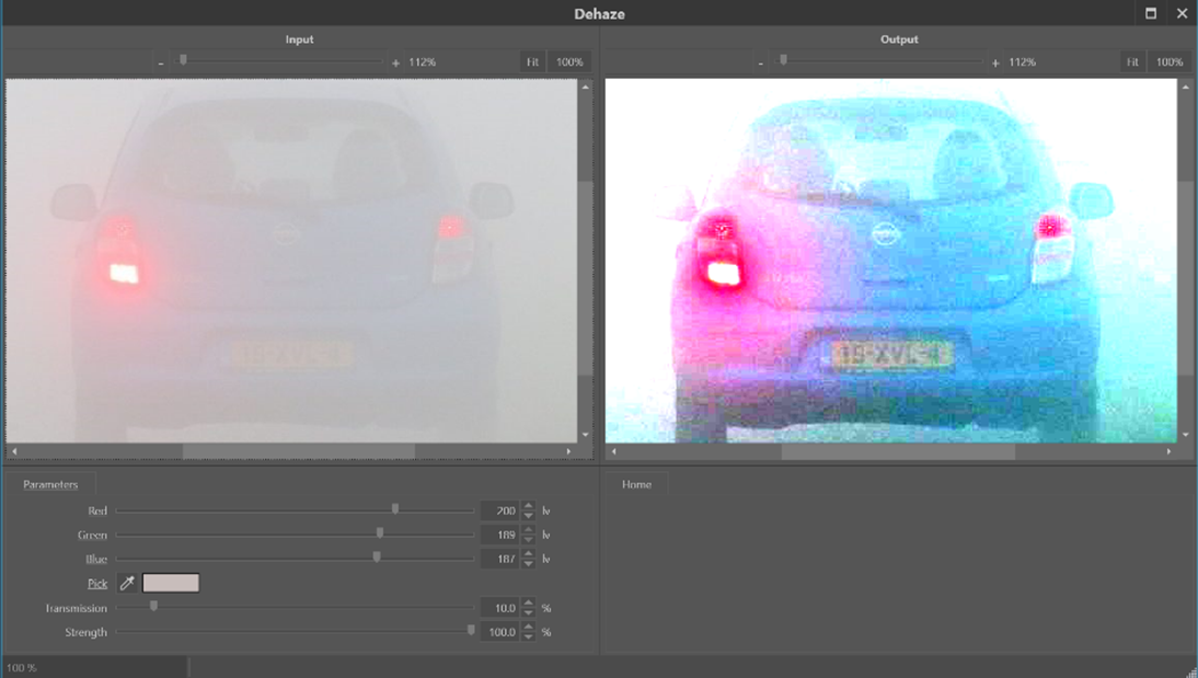
Figure 1: Applying the Dehaze filter to a misty picture. The parameters Red, Green and Blue are the colour components of the selected atmospheric background in the picture. The colour picker ‘parameter’ allows selection of the atmospheric colour by clicking on the picture to the left.

The Transmission parameter is used to tune the distance from the camera that has optimal lighting (see Figure 2 and 3). A lower Transmission value corresponds to the situation where more of the environmental light was lost due to the haze effect before it could be captured by the camera. This is, for example, the case if the object of interest is further away from the camera since, in that case, the light has to travel a longer path through the haze. Finally, the Strength parameter controls the strength of the effect applied to the image.

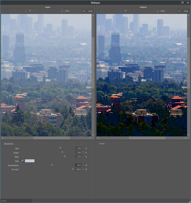
Figure 2: Applying the Dehaze filter on an image with foggy atmosphere. By varying the Transmission parameter, one can select which distance from the camera has optimised levels.

Figure 3: Varying the Transmission parameter over 80%, 60%, 40% and 20% reveals details in the image from front to back.

Selection of the atmospheric colour in a haze is the standard practice in optimising the dehaze filter. However, it can be beneficial to play around by picking different reference colours. Figure 4 shows the result from the dehaze filter, when picking the colour of the back side of the respective cars (solid red arrows), right next to the respective number plates. The bottom image shows the most generally improved image. In this case, the reference color was selected from an area that corresponds to the sky. Although the overall picture is the most appealing, it does not reveal the maximum information about the number plates of the two cars.

Figure 4: By picking a different atmospheric colour from this sandstorm image, indicated by the red arrows, different details are revealed in the situation at the top and bottom. The colours were picked by clicking on the left-side image (solid red arrows).

Conclusion

Although the issues caused by haze are not as impactful as other quality issues, reduction of such early in the sequence of enhancement operations can optimise those which follow. As enhancements are a chain of individual operations, each of which plays a role in improving the image, one should always seek to address all of the quality issues with appropriate tools. Although changes to contrast may improve the effects of haze, the operation is not dedicated to the specific task of haze reduction. It will, therefore, not be as effective as an algorithm designed specifically for the job of haze reduction and may have an unintended effect on other elements of the imagery, such as the introduction of halos. 

REFERENCES

[1]          J. Sumitha, “Haze Removal Techniques in Image Processing,” IJSRD - Int. J. Sci. Res. Dev. Vol 9 Issue 2 2021 ISSN Online 2321-0613, vol. 9, no. 02, Apr. 2021.

[2]          World Meteorological Society, “Haze definition.” Jun. 08, 2023. [Online]. Available: https://cloudatlas.wmo.int/en/haze.html

[3]          K. Ashwini, H. Nenavath, and R. K. Jatoth, “Image and video dehazing based on transmission estimation and refinement using Jaya algorithm,” Optik, vol. 265, p. 169565, Sep. 2022, doi: 10.1016/j.ijleo.2022.169565.

[4]          W. Wang and X. Yuan, “Recent advances in image dehazing,” IEEECAA J. Autom. Sin., vol. 4, no. 3, pp. 410–436, 2017, doi: 10.1109/JAS.2017.7510532.

[5]          Q. Wang and R. Ward, “Fast Image/Video Contrast Enhancement Based on WTHE,” in 2006 IEEE Workshop on Multimedia Signal Processing, Victoria, BC, Canada: IEEE, Oct. 2006, pp. 338–343. doi: 10.1109/MMSP.2006.285326.

[6]          S. Fang, J. Zhan, Y. Cao, and R. Rao, “Improved single image dehazing using segmentation,” in 2010 IEEE International Conference on Image Processing, Hong Kong, Hong Kong: IEEE, Sep. 2010, pp. 3589–3592. doi: 10.1109/ICIP.2010.5651964.

[7]          R. T. Tan, “Visibility in Bad Weather from A Single Image”.

[8]          M.-J. Seow and V. K. Asari, “Ratio rule and homomorphic filter for enhancement of digital colour image,” Neurocomputing, vol. 69, no. 7–9, pp. 954–958, Mar. 2006, doi: 10.1016/j.neucom.2005.07.003.

[9]          X.-W. Yao, X. Zhang, Y. Zhang, W. Xing, and X. Zhang, “Nighttime Image Dehazing Based on Point Light Sources,” Appl. Sci., vol. 12, no. 20, p. 10222, Oct. 2022, doi: 10.3390/app122010222.

[10] Kim Eun-Kyoung Lee Jae-Dong Moon Byungin Lee Yong-Hwan Hardware Architecture of Bilateral Filter to Remove Haze, Communication and Networking: International Conference, FGCN, p129 Springer (2011).

Noise Part 2

Article by James Zjalic (Verden Forensics) and Henk-Jan Lamfers (Foclar).

Introduction

In our previous blog article, we discussed the causes and some possible solutions to noise in digital imagery. In this follow up article, alternative solutions for specific types of noise are presented.

Lowpass Frequency and Wiener Noise

A discussed within our previous article on blur, an image can be represented by its power spectrum. In this spectrum, the image signal is decomposed into a range of high and low frequencies, as demonstrated in Figure 1 a-c. The low frequencies correspond to the slowly varying local average, whilst the high frequencies correspond to both the small details and the inherent noise signal. By suppressing the high frequencies relative to the low ones, the noise signal is attenuated, but at the expense of image detail [1] page 240.

Figure 1: A natural image (a) and its corresponding power spectrum (b). (c) gives a schematic description of the power spectrum in areas (0)-(3). (0) contains the origin (frequency zero) and low frequencies, (1) the higher horizontal frequencies, (2) the higher vertical frequencies and (3) mainly noise and some high frequencies.

The Wiener noise filter [1] page 341, is a very specific implementation of the Wiener deblur filter. In this filter, the blur is assumed to be absent. So, no blur correction is applied, only the noise compensation. Different implementations of the lowpass frequency filters are available, e.g. Ideal, Gaussian and Butterworth. The implementations differ in how the separation/transition between low and high frequencies are handled (see Figure 2).

Figure 2: Filter frequency response of Gaussian (blue), Butterworth (yellow) and Ideal (red) filter kernel.

Denoise

The denoise filter is a noise suppression algorithm that considers the location of contours within an image. A contour is a line that connects points in an image with equal intensity (see Figure 3). The variation of intensity along a contour can therefore be assumed to be caused by noise. Averaging these contour intensity values (see Figure 3 line A) suppresses the noise, but as averaging the perpendicular intensity variations (see Figure 3 line B) will seriously blur the details in the image, it should be avoided. The denoise filter carefully considers the location of both flat intensity regions and the image contours, making it possible to reduce the noise level in the image without causing a loss of detail.

Figure 3: Example of an image contour point P and the direction along the contour A and perpendicular to the contour B.

Median Filter

The median filter ([2] page 108 and [3] page 130), is a noise reduction filter best applied as a solution for impulse noise. For every input pixel, the histogram of a local environment is calculated, and the resulting output pixel is the median value of the local histogram (see Figure 4), thus eliminating  outlier pixel values. Besides a standard implementation of the median filter, Impress also offers the so-called band implementation (see Figure 5). This implementation has an extra parameter entitled ‘Threshold’ that is used to distinguish outlier pixels from ‘normal’ pixels. The filter only replaces the outlier pixels by the local histogram median value, leaving the normal pixels untouched.

Figure 4: The Median filter calculates the median value (37) from local histogram, useful to elimination outline values e.g. in case of impulse noise.

Figure 5: Band implementation using threshold, to select outliers (8, 77) for filtering. Only the pixels that are outside the band will be filtered.

Bilateral Filter

The bilateral filter [2] page 110, is a variant of the lowpass filter. The resultant pixel gets the local weighted average of a small rectangle. However, the weights of the contributing pixel values are not only determined by the distance from the result pixel location (special weight): the larger the deviation of a pixel value from the local average value, the smaller the signal weight will be for that pixel. The total weight for a contributing pixel is the product of signal and special weight (see Figure 6). This approach reduces the undesirable influence of outlier pixels on the local averaging process.

Figure 6: Bilateral filter; the resulting average is determined by the product of spatial and signal weight. This results in the strongest contribution from the pixels close by, excluding outlier values.

Frame Averaging

In cases in which noise reduction is required for a video sequence, it can be accomplished by so-called frame averaging [4] page 32. This is premised on the assumption that the scene is stationary, and thus the only difference between the pixel values from subsequent video frames within the same image coordinates is the temporal fluctuating noise signal. By determining the temporal average for each pixel location, a single image with suppressed noise signal can be constructed (see Figure 7).

Figure 7: Single image Frame Average, the temporal average for all frames in a video.

It should be noted that if the frame averaging is applied to sequences with non-stationary scenes, the result will be a single image with low noise levels that is subject to a degree of blur due to the transitions between the scenes. This blur resembles a motion blur which can be present in images with a long shutter speed time. If the scene is only static for a certain period, preselection of only the stationary part should be used to get a good, blur free, result. If you want to remove the noise from a non-stationary region of interest, one option is to pre-process the imagery using image stabilization to fix the region to a single location for a certain time interval.  Once this has been performed, the frames within the stationary region can be time-averaged. The frames outside the region might exhibit non-stationary behaviour that leads to blur, but these are of little consequence as they are outside of the required region.

Temporal smoothing

When noise exists within a video, the frame average filter only offers a solution in cases where h which the desired region is stationary. Where this is not the case, the so-called temporal smoothing filter [4] page 228 might be useful. Using the box filter from part 1, the average pixel values are calculated from the local neighbourhood of a pixel location in a process that can be described as spatial smoothing. The average pixel value for frame averaging is then calculated for all frames in a video. In contrast, the average pixel value in temporal smoothing is determined over a limited number of subsequent frames (see Figure 8). The weights of the pixel values of the subsequent frames can be constant for a certain interval (box function). Another implementation of this temporal smoothing has weights that become smaller as you go back further in time. The most recent frames contribute the most. A third implementation of temporal smoothing uses the temporal median value over a time range, eliminating outlier pixel values.

Figure 8: Constructing a temporally smoothed video.

Conclusion

As previously stated, noise reduction is always a balance between the suppression of unwanted noise and the preservation of image details. Special situations (such as impulse noise) can be treated with special filters (such as a median filter). Video sequences offer extra options for the reduction of noise,  e.g. frame averaging and temporal smoothing, for stationary and non-stationary scenes, respectively.

References

[1]          William K. Pratt Digital Image Processing, Wiley 2007.

[2]   R. Szeliski Computer Vision, Algorithms and Applications, Springer 2011.

[3]   Sonka M. Hlavac V. Boyle R. Image Processing, Analysis and Machine Vision, Brooks/Cole Publishing Company 1999.

[4] Alan C. Bovik, Handbook of Image and Video Processing Academic Press 2010.

Noise Part 1

Article by James Zjalic (Verden Forensics) and Henk-Jan Lamfers (Foclar).

Problem

Noise is an inherent part of digital imagery, and signal processing in general. It is commonly defined as the undesired region of a signal and in the majority of cases its random nature means that it does not impact the desired region of an image to the degree that misinterpretation of such would occur in isolation. With that being said, if it is not removed and other enhancement processes are applied, it is likely that the visibility of the noise will increase [1], which may then result in issues relating to interpretation. Even if other enhancement processes are not to be applied or there is no risk of misinterpretation, the fact remains that it reduces the overall quality of digital imagery, and so any steps which can be taken to reduce or remove noise are often desirable.

Cause

Noise is most commonly obtained during the acquisition stage, although it can also be added to a signal during any subsequent transmission stages due to channel interference. As the light signal which enters a camera lens must undergo a series of processes prior to being encoded as a digital image or video, each process adds a degree of noise to the original signal, culminating in that which appears visible to us as noise within the final imagery. These processes include the conversion of light to electrons and the amplification of the electronic signal, and the degree of noise is dependent on a number of factors, including the light levels and efficiency of the internal electronics of the capture system. This can be easily evidenced by reviewing low light level captures, as they generally contain more noise than those captured in more brightly illuminated environments as the amount of signal amplification required is higher.

Figure 1: Examples of noise, from left to right impulse, pattern and line noise.

The most commonly encountered types of noise (see Figure 1) are impulse noise (also known as salt and pepper noise due to its speckled black and white appearance), pattern noise and line noise . Impulse noise is characterised by the visibility of random black and white pixels throughout an image, caused by dead pixels in the imaging sensor or the addition of electronic noise prior to encoding. Pattern noise is visible as coloured pixels generated by the variation in the three colour sensors or the analogue to digital conversion process. When there is a composite analogue connection between a camera and a recorder, there is only a single channel available to transmit the data. The colour information is therefore encoded in a high frequency carrier wave, and the signal digitised once it reaches the recorder. The overlap between the high frequency luminance and colour information causes misinterpretation by the frame grabber of the high frequencies as colour which results in colour distortion. This can also occur in black and white captures. Line noise is visible as vertical or horizontal light or dark lines and is generally caused by synchronisation issues in the sensor [2].

Solutions

There are various processes used to remove noise, however, considerations must first be made as to whether the desired signal exists within a video or still image, as although the approaches to each are similar, there can be differences in the specifics.

When noise exists within a video, the possibility exists that a process can be applied to a number of frames in series to increase the signal to noise ratio. For example, if the desired region is stationary (such as the number plate of a parked vehicle), the frames can be averaged, thus reducing the impact of random variations (or noise) between frames. This method is of no use if the desired region is moving as the natural variation between frames would be too great, in which case the exhibit would need to be treated as a still image , unless stabilisation can limit the degree of spatial difference between sequential frames.

The approach for still images is based on a similar theory, but the spatial representation of the image is considered and averaging applied within neighbourhoods of pixels rather than between frames. This is based on the premise that there is expected to be a degree of correlation between neighbouring pixels representing the desired region. In contrast, random noise within said region is uncorrelated with such and is therefore reduced. As the method is based on the assumption that neighbouring pixels are similar, the theory falls down at object edges (or within high-frequency regions) and reduces the sharpness of such [3].

Figure 2: Applying a 3x3 kernel to calculate the local average for three subsequent positions in the image

If one considers that neighbourhoods of pixels 3 x 3 in dimensions (Figure 2) are used for the procedure (square blocks composed of 3 pixels in width by 3 pixels in height), it is the pixel at the centre of this matrix (or kernel) for which a new value is generated. The square then moves one pixel across, and the process repeated. It will continue in this manner (moving down to a new row once the end of the current row is reached) until a new image is created consisting of the new pixel values. Kernels are generally composed of odd numbers of pixels and are centred around a single-pixel (e.g. 3x3, 5x5, 7x7), where the larger the size of the kernel, the more processing power required, and thus, the more noise reduction (and thus loss of feature detail) that will occur. These noise reduction processes are a type of low pass filter as they allow low-frequency information to pass whilst reducing high-frequency information [4].

Conclusion

Noise reduction can improve the overall quality imagery and optimise further processes, but one should always balance the need for a reduction in noise with the associated reduction in object edges (and therefore feature detail). With that being said, there are some approaches that work better than others in maintaining detail, and the next blog in this series will delve deeper into the specific solutions and implementations available for noise reduction in digital imagery.

References

[1]          S. Ledesma, “A proposed framework for image enhancement,” University of Colorado, Denver, 2015.

[2]          J. C. Russ, Forensic Uses of Digital Imaging. CRC Press, 2001.

[3]          R. C. Gonzalez and R. E. Woods, Digital Image Processing, 3rd Edition. Pearson, 2007.

[4]          Mark Nixon and Alberto Aguardo, Feature Extraction & Image Processing. Newnes, 2002.

Authenticity

ARTICLE BY JAMES ZJALIC (VERDEN FORENSICS) AND HENK-JAN LAMFERS (FOCLAR).

Importance of Authenticity

The justice system is built on the principle of fairness, as defined by the term ‘justice’, or the quality of being just, impartial or fair [1]. As decisions within the system are based on evidence, it is essential that all exhibits are accurate representations of what they purport to be, so much so that charges can be brought against any party that attempts to manipulate evidence, regardless of if this is given verbally or submitted for analysis.

We live in a time when the world is dominated by digital imagery, and its advantages to the justice system are clear. It can provide compelling visual evidence of events, something which was not possible just fifty years ago. It is also not subject to the fragility of the human cognitive system, which can bias an account or even omit important elements of such [2]. Despite the inherent advantages of digital imagery to the justice system, in the age of deep fakes and photoshopping the potential for manipulation must always be considered prior to any work being performed, for if later down the line a video is found to be manipulated, all work and inferences drawn from the imagery must be considered unreliable and therefore inadmissible. Although the effects may not be as pronounced, an initial triage of the evidence in the form of a more basic authentication examination can also ensure the most original exhibits are being used for enhancement or analysis, thus eliminating the potential for quality degradation. At the most fundamental level, this could involve analysis to determine the software was used to encode the exhibit, for it is found to be a screen capture or conversion it can be accepted that it is not the most original version. Whether the most original version can be made available is another matter, but it should be an experts duty to be a gatekeeper, doing what they can to ensure the most original imagery available is used.

Defining Authenticity

The term ‘authentication’ is the process of substantiating that the asserted provenance of data is true [3], and as such, an authentication examination seeks to determine if a recording is consistent with the manner in which it is alleged to have been produced [4]. Only by establishing the originality of a recording can it be conclusively accepted that a recording has not been edited, as if this is found to be the case, the possibility of deliberate tampering is eliminated [5]. An artefact that is consistent with an edit may have an innocent explanation, but a lack of evidence with regards to editing cannot be considered to be proof that editing has not taken place without establishing that the recording is an original. As the term ‘original’ is relative to the source, the source which is being considered must first be defined based on information provided. For instance, a very basic example would be if a recording is provided which is purported to have been captured using a CCTV system, but the content contains a recording of a monitor displaying the CCTV by a mobile device, it can be accepted that it is inconsistent with an original recording. The potential, therefore, exists that the recording displayed on the screen has been manipulated using video editing software and is therefore providing a false account of the events that occurred.

Now imagine the same scenario, but the recording content is consistent with the capture from a CCTV system. Further analysis is therefore required, which could be in the form of a review of the metadata to determine if details of the software used for encoding the recording are present within. These examples can be performed using freeware suites in under 30 seconds, but are extremely basic and thus are unlikely to reveal any traces of editing if the would-be manipulator has some knowledge of digital imagery. It is, therefore, essential that further techniques are utilised to ensure edited recordings do not slip through the net.

MANDET

Mandet is a software tool for manipulation detection in images and video and provides a broad range of different tools. One of the features is the image content filtering which searches for statistical deviations within the image or video frame (Figures 1 and 2). It also has video trend analysis, which searches for statistical deviations in a specific extracted signal through the whole video. The DeepFake detector is also one of the unique features. Next to the content filtering/analysers, it also includes a hexadecimal viewer in which a file can be investigated at a byte level. Furthermore, it contains metadata extraction, camera ballistics, and some basic tooling.

While the job of searching for manipulations within imagery is a time-consuming job, the software is developed in such a way that it works as efficiently as possible. It is important that the authenticity of an image or video file is determined, but to do this, the tools used to perform analysis should be as efficient as possible, considering the amount of imagery used in forensic cases. Mandet is a tool that provides this in a forensically sound way by automatically generating a working copy and calculating the hashes of the files which will be visible in the report.

It is also possible to do a deep dive into the functionality. Many of the filters have parameters that can be adjusted, and the video trend analysers provide a graph from the derived signal and its automatically determined thresholds.

Figure 1: With two button clicks an overview of different filter results is generated

Figure 2: Derived data being visualised

Conclusion

It is of the utmost importance that imagery presented within the justice system can be accepted as an accurate account of what it purports to represent, as it is evidence that triers of fact base decisions and which defendants are convicted or released upon. No party within the system is better placed to opine on matters of authenticity than a digital imagery examiner, and so it is their responsibility to do what they can to prevent edited imagery from reaching the courtroom.

References

[1]          Merriam-Webster, “justice.” [Online]. Available: https://www.merriam-webster.com/dictionary/justice.

[2]          A. Memon, S. Mastroberardino, and J. Fraser, “Münsterberg’s legacy: What does eyewitness research tell us about the reliability of eyewitness testimony?,” Appl. Cogn. Psychol., vol. 22, no. 6, pp. 841–851, Sep. 2008, doi: 10.1002/acp.1487.

[3]          SWGDE, “Digital and Multimedia Evidence Glossary Version 3.0.” Jun. 20, 2016.

[4]          SWGDE, “Best Practices for Digital Forensic Video Analysis,” p. 18, 2018.

[5]          A. J. Cooper, “Detection of copies of digital audio recordings for forensic purposes,” PhD Thesis, The Open University, 2006.

Proficiency

Article by James Zjalic (Verden Forensics) and Henk-Jan Lamfers (Foclar).

Introduction

As the probative value of forensic science is intrinsically linked to the reliability of such, it is essential that the performance of tools used, methods implemented and application of such by examiners is consistent from case to case. Without assurance of these factors, how can the trier of fact be sure that non-crucial information has been lost during an imagery enhancement? In the first instance, it must be demonstrated that the tools used are appropriate and function as expected, because although an examiner may be proficient if increasing the brightness by 5% using a fader results in differing amounts of brightness depending on the day or the format of the imagery being enhanced, the outcome may be unreliable. Confidence in the tools can be obtained through validation, a process which will be covered in a future article. In the second instance, the method itself must be reliable, as the tool may function as expected and the examiner may be competent, but the ability to follow a method correctly will be of no use if the method produces misleading, poor or unstable results. Finally, the examiner must be proficient in performing the method, a factor which can be evidenced by them taking part in some form of controlled assessment, or ‘proficiency test’ [1].

Proficiency Tests

Proficiency testing: The determination of the calibration or testing performance of a laboratory or the testing performance of an inspection body against pre-established criteria by means of interlaboratory comparisons [2].

The advantages of participation for the organisation include, but are not limited to:

• Training of personnel;

• Promoting baseline competency;

• Improving laboratory practices;

• Identify risks;

• Measure error rates.

The tests can be blind (where the source of the tested sample is not revealed until after the test, and the examiners are not aware they are in a test), or open (where the source is known, and the examiner understands they are being tested). They can also be internal, and thus developed by the organisation, or external, and developed by a party with no vested interest in the result. As blind tests mean the examiner performs as they would in a real case, and their creation by an external organisation mitigates against any biases, blind tests are held in the highest regard. One method to implement such is for the test to be submitted in accordance with casework, allowing the examiner to believe it to be such and acts in their normal manner.

Where the performance is poor, the reasons for such must then be investigated. Did the examiner deviate from the method? And if so, was the deviation accidental due to incompetence or deliberate? [3] Or did the examiner conform to a poor method? The results can then be used to determine if the methods should be improved or abandoned and assess whether further staff training is necessary [4].

Interlaboratory Comparisons

Interlaboratory Comparison: The organisation, performance and evaluation of calibration/tests on the same or similar items by two or more laboratories or inspections bodies in accordance with predetermined conditions [2].

These are often performed instead of formal proficiency tests for a number of reasons, including:

• Lack of proficiency testing availability;

• The unreasonable burden it would place on the laboratory;

• The low number of laboratories within the sector.

They can involve a large number of labs, or few. When there are fewer than seven laboratories taking part, the ILC is classed as a ‘small ILC’, which can come with its own difficulties in interpretation of results due to the limited number of such [5].

Generally, for these types of comparisons, there would be an organiser and a number of participants. The organiser takes the responsibility of creating the test and dataset, and then analysing and reporting the results. The participants are those who take part, which can include the organiser.

There are various factors for consideration when developing an interlaboratory comparison exercise, such as the types of data (qualitative or quantitative), how the data is provided (in a series round-robin type manner where each participant passes it onto the next or simultaneously) and whether the tests will be continuous or a one-off test.

In imagery forensics tests would generally be simultaneous, owing to the nature of digital data for bitstream replication. Quantitative tests may be those for which a quantitative result is possible, such as rewrapping or conversion, whereas qualitative would be enhancements and morphological comparison exercises [6].

ILC’s must always be performed using the laboratories own documented methods and procedures, and any unexpected performances are classed as non-conformities [7]. As the test is a comparison, the goal is to determine the performance of the laboratory relative to other laboratories. They do not, therefore, explicitly require known, expected outcomes (which is not possible with qualitative disciplines), but is of benefit where suitable, such as those with quantitative outputs.

Summary

Lay people place a strong weighting on expert opinion, and so it is vital that it is as reliable as possible. In order to ensure reliability and improve procedures, a combination of validation, interlaboratory comparisons and proficiency tests should be implemented within all forensic laboratories quality management systems.

References

[1]  J. J. Koehler, “Proficiency tests to estimate error rates in the forensic sciences,” Law Probab. Risk, vol. 12, no. 1, pp. 89–98, Mar. 2013.

[2]  United Kingdom Accreditation Service, “TPS 47 - UKAS Policy on Participation in Proficiency Testing.” Feb. 04, 2020.

[3]  R. Mejia, M. Cuellar, and J. Salyards, “Implementing blind proficiency testing in forensic laboratories: Motivation, obstacles, and recommendations,” Forensic Sci. Int. Synergy, 2020.

[4]  W. E. Crozier, J. Kukucka, and B. L. Garrett, “Juror appraisals of forensic evidence: Effects of blind proficiency and cross-examination,” Forensic Sci. Int., vol. 315, 2020.

[5]  European Accreditation, “Guidelines for the assessment of the appropriateness of small interlaboratory comparisons within the process of laboratory accreditation.” 2018.

[6] R. M. Voiculescu, M. C. Olteanu, and V. M. Nistor, “Design and Operation of an Interlaboratory Comparison Scheme.” Institute for Nuclear Research Pitesti, Romania, 2013.

[7] Forensic Science Regulator, “Codes of Practice and Conduct FSR-C-100,” no. 5, 2020.

De-Blur

Article by James Zjalic (Verden Forensics) and Henk-Jan Lamfers (Foclar).

The Problem

Blur is a historical problem for which solutions have been studied over a number of decades. Its root cause is the inability of an imaging system to focus on objects on an image plane at the same time, or relative motion between a camera lens and an object during exposure. The uncontrolled and varying conditions of forensic imagery can result in both of these causes being realised, and thus it is extremely common for both images and video to require some form of de-blurring within the sequence of enhancement operators applied to recover high-frequency information, and thus detail.

Cause

The issue itself is caused by the convolution of an original image with a point spread function (PSF; the output of a system in relation to a point source input). Examples of types of blur within forensics include:

• Linear Motion Blur.. The result of relative motion between a camera viewpoint and the source during exposure time. It can be worse in low light conditions where longer exposure times are required.

• Rotational Motion Blur. The result of the relative motion when a camera approaches an object at high speed.

• Defocus. Objects near the camera are sharp, whereas those in the distance are blurred.

• Radial blur. A type of defocus caused by the inherent defect of an imaging system such as a single lens, characterised by an image which is sharp at the centre and blurred as the distance from the central plane increases.

(Zhang and Ueda, 2011)

In a worst-case scenario, the difficulties are compounded when a number of the above exist, for example where the camera is in motion, and the subjects appear at different distances from the camera lens moving in different directions. When it is considered that other issues may also exist, including those related to noise and colours, it is likely that the quality of an image will be limited by such.

Theory

When an image is captured, the lens does not focus a single point to a corresponding point on the sensor, and thus the colour information pertaining to an object is diffused from a central region. The magnitude and direction of this spread can be considered to be the point spread function.

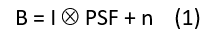
Blur is caused by the convolution (Ä) of the latent (or true image) with the point spread function, as below, where B represents the blurred image, I the latent image, and n the noise.

(Pan et al., 2019)

Solution

In cases where the PSF is known, such as the Hubble telescope, it is possible to de-convolve the PSF from the provided image to obtain the original image. In most practical applications, including forensics, the PSF is not known as the content of the capture cannot be predicted. The presence and correction of blur is therefore known as a blind de-convolution process, in which a sequential approach is utilised by first estimating the PSF and then de-convolving the blurred image. The estimation process is generally iterative, in which estimation is made followed by adjustments. The most common method is to model the PSF is a shift-invariant kernel (Bar et al., 2006). A key limitation as it applies to forensics is that this model assumes that the degree and direction of blur is uniform across the image, which is not necessarily the case (again, consider two subjects running in opposing directions). The selected PSF will therefore either be a compromise and thus the blur will not be as reduced as much as it could be, or will reduce the blur pertaining to one element whilst likely increasing the blur relating to the other (Hu and Yang, 2015; Russ, 2001).

The process of reducing blur is known as de-blur, and considerations for its position in the order of operations must be made. As sharpening increases the contrast between high-frequency regions, and blur reduces high-frequency information, the result of sharpening a blurred image would be sub-optimal. It must also be considered that colours within a blurred image are diffused throughout due to the convolution with the PSF, and so colour adjustments cannot be accurately applied. It is therefore recommended that any de-blur process is performed prior to these operations (Ledesma, 2015).

Implementations

In Impress a number of different types of de-blur filters are available [7], [8], including for linear motion, general misfocus, and custom de-blur. The operator has to select the blue filter, which is most appropriate for the image of interest. The algorithm used for all de-blur filters is the Wiener filter, with differences between the above-mentioned de-blur filters being caused by the shape of the PSF used by the Wiener filter. To be able to explain the way is filter works, first, the power spectrum has to be introduced.

Power spectrum

The power spectrum is an alternative way to characterise a signal. For example, a sinusoid shaped audio waveform can be described as a single frequency (Figure 1).

Figure 1: Temporal audio signal and its corresponding power spectrum (frequencies).

A one-dimensional time signal is decomposed in one or more frequencies (in this case a single frequency), displayed in the one-dimensional power spectrum. Similarly, an image with two spatial coordinates in pixels can be decomposed into a two-dimensional power spectrum. This is shown in Figure 2, where an image with a sine wave results in a power spectrum with two main frequencies inside the blue ellipses. The origin is indicated by the yellow ellipse (frequency value zero), which corresponds to the average brightness level in the image. The outer areas of the power spectrum correspond to the high frequencies in the image. The high frequencies represent both noise signal and the fine details of the image (sharp contours). Notice that the axis in the power spectrum is rotated over 90 degrees relative to the direct space image coordinates. A natural image can be considered to be build up by many sine waves of different magnitudes (amplitudes), frequencies, directions and starting points (phase). The power spectrum of a natural image is, therefore, more complex, see for example Figure 3.

Figure 2: Image with a) (vertical) sinus intensity wave and b) corresponding power spectrum.

Figure 3: A natural image (a) and its corresponding power spectrum (b). (c) gives a schematic description of the power spectrum in areas (0)-(3). (0) contains the origin (frequency zero) and low frequencies, (1) the higher horizontal frequencies, (2) the higher vertical frequencies and (3) mainly noise and some high frequencies.

The mathematical transformation to calculate the audio power spectrum going from time (seconds) to frequencies (Hz) is the Fourier transform. Similarly, the two-dimensional Fourier transform is used to calculate the power spectrum of an image, going from direct space pixels (Figure 2a, 3a) to frequency pixels (Figure 2b, 3b).

Fourier transform

This Wiener filter uses the Fourier transform  (and  its inverse transform) as a mathematical tool to estimate the latent (sharp) image I from the blurry image B. The trick is to transform the equation (1) to its Fourier equivalent:

This way, the complex convolution operation (Ä) for direct space pixels changes into a simple frequency pixel by pixel multiplication (x). This equation can be solved for I if PSF and n are known, giving:

with SNR being the signal-to-noise ratio of the image.

The final step is to inverse Fourier transform the result (3) to recover the latent image:

Linear motion deblur

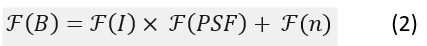
During the shutter time of the recording of a single frame or still image, the camera or object(s) of interest or both can move. If the motion is fast relative to the duration of the shutter time, this results in so-called blur streaks. To compensate for the effect the Blur parameter should have a value which corresponds to the length of the blur streak. The Angle parameter should correspond to the angle between the streak and the horizontal axis. Both parameters control the shape and extent of the PSF function of formula (1).

Figure 4: Example of a blur streak due to linear motion blur.

In real-life cases, the blur streaks (Figure 4) might be less obvious to find, see, for example Figure 5 and 6. The noise signal is estimated from the outer areas of the power spectrum. In Figure 7 this corresponds to the non-red areas. With the Noise Area parameter, which acts as a cut off between signal and noise frequencies, these areas can be adjusted. If the image contains many high-frequency features, decreasing the parameter value will help to preserve these. The Noise parameter allows the operator to tune the strength of the noise compensation of the filter. In Figure 8, the de-blur result on the front end of the taxi is displayed for different values of the so-called threshold parameter. This parameter suppresses wave-like distortions in the result images. If the parameter is chosen too large, the de-blur compensation is not so effective anymore. The color parameter enables the de-blur on the luminance or individual colour channels.

Figure 5: example of linear motion de-blur.

Figure 6: Taxi left front wheel (a) in detail (c), which reveals the linear motion blur present by a subtle blur streak indicated by the Cyan line in (b) and (d).

Figure 7: the power spectrum of the filter input image of Figure 4. The noise levels are estimated from the area’s outside the red area.

Figure 8: de-blur results with (a) original detail, (b),(c) and (d) threshold values of 10, 245 and 1000.

Misfocus

Examples of misfocus are shown in Figure 9 and 10. The blur effect has the shape of circles. The misfocus de-blur or defocus filter should have a Blur parameter value corresponding to the radius of the blur circles.

Figure 9: Blur circles due to mis-focus. The Cyan line indicates the diameter of the blur kernel PSF in the image.

Figure 10: Example of a misfocused image.

General de-blur

The general or thermal de-blur filter uses a Gaussian PSF function (formula (1)). The Gaussian function can, for example, be used to model atmospheric turbulence accurately. This filter is also very useful for post-processing of super-resolution images, and as a general sharpen filter in cases where the blur source in the image is the result of many blur sources. The parameter settings are similar to the misfocus de-blur filter.

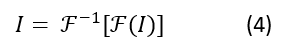
Custom de-blur

In case the blur effect in an image is caused by non-linear motion or a complex composition of multiple blur types, one can apply the so-called custom de-blur filter. In Figure 11 an example is shown of a non-linear accelerated motion. The motion blur, in this case, is very complex, and so could not be modelled by a curved line, since the motion was accelerated, resulting in intensity variations along the curve. If the blur kernel feature can be isolated, it can be used to compensate for the complex blur pattern it represents. Ideally, the blur kernel is in the filtered image changed into a single dot. Therefore, if one knows that some blurry feature in an image should originate from a point-like shape, one can use this blurry feature for extraction of the blur kernel using the custom de-blur filter. The above extraction procedure is independent of the complexity of the blur pattern in the image. The only condition is that it should be possible to separate the blur feature from the background. To further facilitate this process, extra ‘drawing’ options (Figure 11 b) are available to retouch the extracted blur kernel. The hash of the extracted kernel image is included in the processing log to guarantee reproducibility.

Figure 11: Example of a complex blur kernel (b) extracted from the blurred image (a). In the result image (c) the blur kernel approximates a single dot (d).

Conclusion

Although the requirement for assumptions to be made in relation to the unknown point spread function prior to de-convolution can cause limitations in the results of de-blurring, when a good estimate is achieved the results can be highly effective.

References

[1] Bar, L., Kiryati, N., Sochen, N., 2006. Image Deblurring in the Presence of Impulsive Noise. Int. J. Comput. Vis. 70, 279–298. https://doi.org/10.1007/s11263-006-6468-1

[2] Hu, Z., Yang, M.-H., 2015. Learning Good Regions to Deblur Images. Int. J. Comput. Vis. 115, 345–362. https://doi.org/10.1007/s11263-015-0821-1

[3] Ledesma, S., 2015. A Proposed Framework for image enhancement. University of Colorado, Denver.

[4] Pan, J., Ren, W., Hu, Z., Yang, M.-H., 2019. Learning to Deblur Images with Exemplars. IEEE Trans. Pattern Anal. Mach. Intell. 41, 1412–1425. https://doi.org/10.1109/TPAMI.2018.2832125

[5] Russ, J.C., 2001. Forensic Uses of Digital Imaging. CRC Press.

[6] Zhang, Y., Ueda, T., 2011. Deblur of radially variant blurred image for single lens system. IEEE Trans. Electr. Electron. Eng.

[7] Sonka, M., Hlavac, V., Boyle, R., 1999. Image Processing, Analysis and Machine Vision, p106. Brooks /Cole Publishing Company.

[8] Bovik, A.C., 2010, Handbook of Image and Video Processing, p173. Academic Press.

Look Up Tables

Article by James Zjalic (Verden Forensics) and Henk-Jan Lamfers (Foclar).

The Problem

Due to the inherent issues caused by uncontrolled capture environments, the intensity values within a digital image can cause the colours to appear unnatural and not accurately representative of those within an environment. . In most cases imagery could benefit from an adjustment to characteristics such as the brightness or contrast, or balancing of the histogram using operations such as normalisation or equalisation. Although there are nicely presented applications which make these operations simple, all utilise Look Up Tables [1] (or LUT’s) behind the scenes to make these changes, so by directly manipulating the LUT (or a representation of such as a plot), the greatest level of control and optimal results can be achieved.

The Cause

The general causes of issues relating to poor representation of a scene by digital imagery have been covered in previous articles, so will not be covered here.

Theory

Look Up Tables are essentially tables containing the output result for each possible input, so in order to transform one input value to a predefined output value, the computer ‘looks up’ the tabulated result. For example, if one considers a grey-scale 8 bit image, a brightness adjustment of 10 intensity values will result in a table that contains each possible input (from 0 – 255), with each output (the original input value plus 10). Rather than adding 10 to each input value independently, LUT’s are efficient as all values are already stored within the table (see Figure 1). LUT’s can be defined by their dimensionality, with the example being classed as 1-D as it takes one input and applies one operator to it (+10) to result in one output.

Figure 1 : Example of a section (0-10) of a LUT that implements adding 10 to each input value to get the output value.

Although one-dimensional LUT’s implementations are suitable for basic operators that can be represented by a single variable, such as brightness, gamma and contrast, not all parameters can be characterised by a single variable [2]. In these cases, a 3-D LUT is more suitable, as they are more accurate and flexible, and are therefore used for applications such as colour space transforms. Due to the large number of coordinates required, 3-D implementations use interpolation to decrease the computational power required. For more information relating to such, please visit the previous article on re-scaling.

As RGB images consist of three layers, three 1-D operators are used (one per channel) to achieve the best results [3].

Implementations

When performing LUT based operations on a grey-scale 8 bit image, the range of possible values is 0-255. For this type of image, the number of entries in the LUT is therefore 256. In Impress, images used for filtering are represented by values which are double-precision float. Each colour channel (red, green and blue) of a single pixel is therefore represented by a 64 bit number. This gives the opportunity for higher precision calculations when compared to 8 bit numbers as when multiple filters are used accumulative rounding errors can occur which can seriously deteriorate the final result. To limit the number of entries, the LUT is a 256 x 256 array for each colour channel, and intermediate pixel values are calculated through interpolation.

The options available within the Curves [4] filter in Impress are presented in the detail window of the filter shown in Figure 2. The window offers a side-by-side display of the input and output image of the filter, and the histogram of the input image is also displayed. By switching on the region of interest inspector parameter ROI, the histogram shows only the levels inside the red rectangle. This option is very useful for images containing areas of different lighting. The current values inside the lookup table are plotted on top of the histogram. The shape of the plotted curve can be controlled by positioning the  ‘control points’, and their positions can be changed by dragging the thumb in the graph or by changing in the listing on the left, which is convenient for reproducibility. The type of interpolation curves between the control points is controlled by the Curve parameter. The curves can be either a linear or spline interpolation (see Figure 3). The LUT based filters, e.g. Stretch, Equalise, Gamma and Curves all have the option to process the individual colour channels, allowing colour imbalance compensation in images (Color parameter) by adding three filters working on the individual colours.

Figure 2: Curves detail window.

Figure 3: LUT with linear curves (top) and spline curves (bottom) between the control points.

Conclusion

Understanding the operations that take place behind the scenes when a brightness or contrast adjustment is made to digital imagery gives the user the opportunity to manipulate the Look Up Tables directly, thus providing greater control and operations that are highly specific to the image being processed that can lead to better overall results.

References

[1]  Matt Pharr, “Chapter 24: Using Lookup Tables to Accelerate Color Transformations,” in GPU Gems 2, Nvidia, 2015.

[2]  Mark Nixon and Alberto Aguardo, Feature Extraction & Image Processing. Newnes, 2002.

[3]  Charles Poynton, Digital Video and HDTV: Algorithms and Interfaces. Elsevier, 2007.

[4]   M. Sonka, V. Hlavac, R. Boyle, Image Processing, Analysis and Machine Vision p59, Brooks / Cole Publishing Company , 1999.

Re-Scaling

Article by James Zjalic (Verden Forensics) and Henk-Jan Lamfers (Foclar).

The Problem

When reviewing digital imagery, the scale of such presented to the user can make it difficult for interpretation, especially if in cases where the pertinent object or region is at a distance from the camera lens. This can affect both examiners and end-users a like, and while an examiner has control over any effects that increasing the size may have through the use of validated software, the end-user will likely increase the size of any imagery to fit their computer monitor and apply magnification without understanding the impact of such on the content.

Re-scaling is an operation used to change the size and sometimes the orientation of digital imagery to aid in interpretation [1].

The Cause

The need for resampling essentially stems from the inability of the eye to reliably interpret regions within digital imagery due to the size. The reason for small features generally fits into one of three categories:

1.       The resolution of the imagery is poor.

Where the resolution is low, the representation of regions within will also be low, and as such, the features will be difficult to interpret.

2.       The region of interest is at a distance from the camera lens.

Although the resolution of the overall capture may be good, the number of pixels used to represent the region is low due to the distance of such from the camera lens.

3.       The region of interest is captured at an unnatural orientation.

On occasion, features can be captured from a perspective which is inconsistent with that expected, for example, a vehicle captured at a 90o orientation which is therefore displayed vertically rather than horizontally.

Re-scaling of the imagery is of paramount importance to allow a reliable judgement to be made, as the quality of the content can become both easier to view, and artefacts caused by pixel boundary edges can appear reduced. With that being said, caution must be taken as any re-scaling operation which increases the size or rotates the imagery on a non 90-degree axis can only result in a reduction in the information within an image. Re-sampling cannot increase the resolution of a region, or the information within, as the data has not been captured in the first place.

Theory

Re-scaling (or resampling) is the process of transforming a discrete image to a new set of coordinates through interpolation (the use of known data to estimate values at unknown locations) [2].

There are a variety of interpolation algorithms available, and the selection of such is highly dependent on the application. All re-scaling processes are based on two general steps:

1.       The interpolation of a discrete image to a continuous image;

2.       The sampling of the interpolation image to the new grid.

The most commonly known types of interpolation [3], [4] used for image re-scaling can be categorised based on the number of known data values used to estimate each new values, as follows:

Nearest Neighbour – Uses a single value, where the value of the new pixel is taken from the value of the nearest existing pixel. For one- and two-dimensional examples see Figure 1a and Figure 2a.

Linear – Uses two values either side of the new pixel (see Figure 1b), where the value of the new pixel is taken from the mean of the values of the existing pixels.

Bilinear – Uses four values by implementing linear interpolation on both the horizontal and vertical axis (see Figure 2b).

Bicubic – Uses the sixteen nearest pixels by using the four-pixel values at each of the corners of the pixel, as well as the four-pixel values at each of those pixels corners.

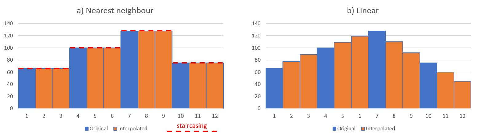
Figure 1: one dimensional example of interpolation (3x scaling) of data with a) nearest neighbour interpolation and b) linear interpolation. The red-dotted lines show the so-called staircasing effect.

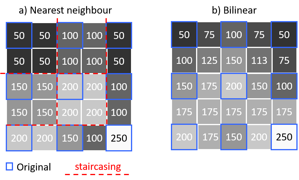
Figure 2: two dimensional example of a grey level pixel interpolation (2x scaling) with a) nearest neighbour interpolation and b) bilinear interpolation. The original pixel values are indicated by the blue borders. The red-dotted lines show the so-called staircasing effect.

Solution

One of the core principles of forensics is to maintain the integrity of evidence [5], and this should be taken into account for all processes from capture to processing. In light of this, several of the interpolation methods must be used with extreme caution, and as the type of interpolation can change the content in different ways, the type used should always be documented within working notes and the final report to ensure reproducibility and transparency. For instance, if one examiner uses bicubic interpolation and other nearest neighbour, the new pixels introduced in each will vary, opening up the potential for differences in interpretation of the same source imagery. With that being said, the algorithm used is of less concern when the imagery is for presentational purposes only, such as when using markers to indicate the movement of a subject within an environment.

As nearest neighbour uses the values of pixels already with the environment rather than create new values from the mean of surrounding pixels, this is the safest option for any imagery which will be used for interpretive purposes. The disadvantage is the staircasing (see red dotted lines in Figures 1 and 2) effect it can have on edges due to the coarse disparity between neighbouring pixels, and the shift in the position of pixel locations. For example, if the locations of new pixels are halfway between the existing pixels, the image will be shifted by half a pixel. Best practice is to resample to a coordinate system with sample spacing that is an integer factor of the original, so the resampled data reproduces the original image.

Implementations

Interpolation techniques use different mathematical functions to interpolate the pixel values, and as such, the number of neighbouring pixels that are used to calculate the result value differ. The local neighbourhood used to calculate the interpolated value can be characterised by a pixel radius. The interpolation techniques for scaling available in Impress [6] are listed in Table 1.

Table 1: available interpolation techniques in Impress

Figure 3: example of scaling: a) original image with region of interest, b)nearest neighbour 10x, c) bilinear 10x and d) Lanczos 10x.

Multiple interpolation techniques are added because of the different characteristics of the resulting images. In Figure 3 an example is shown of three interpolation techniques. From the image it becomes clear that different techniques can produce images of varying degrees of smoothness. Depending on the image content and personal preference a specific technique can be selected.

Figure 4: sharpening is often used to compensate for the blurriness introduced by the scaling. Care should be taken to use the right interpolation in combination with the sharpening as is shown with a) Bilinear and b) Bicubic spline.

The blurriness introduced by the scaling can be compensated by using a sharpen filter after the scaling. Care should be taken to select the right interpolation and the strength of the applied sharpening. Figure 4 shows an example of combining scaling and sharpening. The strong sharpening starts to emphasise artefacts introduced by the interpolation in case of bicubic spline (Figure 4b). In case of bilinear interpolation (Figure 4a), using the same sharpening, the result is much worse.

Figure 5: unlocking the aspect ratio allows the user to set a different scale for the horizontal and vertical axis. On the left the original footage (with ROI) is shown. On the right the aspect ratio corrected image is shown. The scaling filter parameter setting is shown in the bottom-middle.

The aspect ratio of an image is the ratio of width and height (width / height). In some cases an image do not give a good representation of objects from the real world in the image, because the aspect ratio is incorrect (see Fig.5). This can be the result of the recording technique or partially corrupt image data. The scaling filter can be used to adjust the image dimensions to better fit the real world aspect ratio. The operator has to unlock the aspect ratio (Fig. 5), in which case the horizontal and vertical scaling factor can be set independently.

Conclusion

Prior to selecting an interpolation algorithm, the application of the final product should be considered, and a decision made on the impact of the processing on the final interpretation. For tasks which require interpretation, it is always best to urge on the side of caution and use nearest neighbour to ensure no new information is generated and added to the image, but for presentational purposes, the selection is of less concern.

References

[1]          N. A. Dodgson, “Image resampling,” University of Cambridge, Cambridge, UK, 1992.

[2]          Rafael C. Gonzalez and Richard E. Woods, Digital Image Processing, 3rd Edition. Pearson, 2007.

[3]          A. Suwendi and J. P. Allebach, “Nearest-neighbor and bilinear resampling factor estimation to detect blockiness or blurriness of an image,” J. Electron. Imaging, vol. 17, p. 16.

[4]          J. Anthony Parker, Robert V. Kenyon, and Donald E. Troxel, “Comparison of Interpolating Methods for Image Re-sampling,” IEEE Trans. Med. Imag., no. 1, Mar. 1983.

[5]          ACPO, “ACPO Good practice guide for digital evidence,” Mar. 2012.

[6]          Bovik Alan C. Handbook of Image and Video Processing, p33 Academic Press (2010).

Sharpening

Article by James Zjalic (Verden Forensics) and Tom Klute (Foclar).

The Problem

Digital imagery can often suffer from a relatively poor focus on the feature of interest, making it difficult to interpret the true characteristics of such. For example, is an object held in the hand of a subject a knife or a phone? Increasing feature detail can aid in allowing more reliable interpretations to be made and improve imagery for general presentation purposes, even if the feature characteristics are already visible.

Sharpening is an operation used to highlight transitions in pixel intensity values and thus, the visual separation between feature edges.

The Cause

The need for sharpening essentially stems from the poor separation between features within digital imagery. As digital imagery is finite, the analogue to digital conversion is imperfect and so in regions of transition within the dimensions of single pixel neither colour is represented correctly, resulting in blur [1]. This is further compounded by other events, such as::

• Compression. When digital imagery is compressed, high-frequency detail is attenuated, and in some instances completely removed, depending on the encoding format and degree of compression applied. This is to aid in smaller file sizes as data as reducing unique values through replication of the pixel intensity values of similar regions, the less information which has to be stored.

• Camera movement. When cameras move (either through camera shake or manual movement), features are convoluted when represented as pixels leading to little separation.

• Movement with the scene. When there is movement within a scene (for example an individual running), the features are convoluted as with camera movement.

• Image processing artefacts .The application of a deblur operation to remove noise within an image can reduce the disparity between local pixel intensity values, and thus reduce the contrast at edges.

• Camera lens settings. A camera lens which is not properly configured for the scene which it is capturing can cause lens blur by convolving pixels which represent objects within a scene

• Point Spread Function. The point spread function relates to the spreading of light from a point source, which can result in the source covering a wider range of pixels than it should to represent the environment correctly, resulting in convolving pixels, as above [2].

• Anti-aliasing. Cameras tend to employ anti-aliasing filters which can cause Moir patterns in fine detail regions, resulting in edges which are less defined.

  In the best-case scenario, a subject will be stationary, and the compression is the only factor reducing the disparity between local pixel values (and thus visual sharpness). In the worst scenario, all of the above factors are present, which in some cases can lead to imagery which no amount of sharpening can improve.

Theory

Sharpening is achieved through spatial differentiation, which is essentially the opposite of the pixel averaging applied when blurring. It enhances edges and other discontinuities throughout an image, including random noise (which is classed as differences in intensity between a pixel and its neighbour and is expected to be spatially uniform). For this reason, noise must be removed prior to sharpening. The operation emphasises regions in which there are rapid transitions in intensity and de-emphasises those with slow transitions. Edges are often ramp like transitions in intensity, whilst the body of an object is usually a generally consistent intensity which occupies a small range (see Fig. 1).

Figure 1: Intensity range of the inside of an object is smaller than the range of the border area.

All sharpening functions are high pass filters as they remove low frequencies (slow transitions between pixel intensity values) while preserving high frequencies (rapid transitions between pixel intensity values.

Care should always be taken when performing sharpening operations as a) over-sharpening can create unnatural representations of fine details, which can lead to halos of brightness around edges and b) it can increase noise within an image which leads to a reduction in clarity (see Fig. 2). To mitigate against the occurrence of halos, the examiner should always compare the input and output to achieve a balance of a natural representation of the object while increasing the clarity. To prevent the second, sharpening should always be performed after de-noising, and should usually be the last processing operation performed. The application of a sharpening process always requires a balance between managing background noise whilst increasing the definition of feature edges.

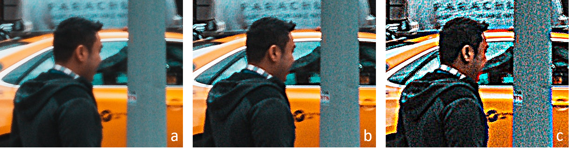
Figure 2: a) original, b) sharpen and c) over-sharpening increasing noise and halo's at the edges of objects.

Solution

Unsharp masking is one of the oldest methods for sharpening the contents of an image. The process subtracts an unsharp (or blurred) version of the original image from the original, causing intensity transitions to become emphasised by producing greater local contract whilst maintaining the overall variation brightness [3], [4]. Within digital imagery, the process is as follows:

1. Make a copy of the original imagery and apply a gaussian blur;

2. Subtract the blurred imagery from the original, resulting in a ‘mask’;

3. Add the mask to the original image.

The amount of subtraction applied determines the degree of sharpening, and this is often the only variable which the user needs to manipulate to ensure optimal results. The drawbacks of the method are that it is extremely sensitive to noise due to the linear filter used, and enhancements high contrast region more than lower contrast regions. This can be an issue if the desired area for enhancement is of a moderate contrast in comparison to other areas [5]. Over-sharpening can be identified by jagged edges and increase levels of noise within an image.

A second method is the use of a kernel, which is a matrix of numbers used to generate new pixel values based on a weighted average of the surrounding pixels. The kernel size and composition can be adjusted to result in differing degrees of sharpening by increasing the difference between pixels [6].

All sharpening processes have to be performed on a converted colour space, as if applied directly to an RGB representation the value of each colour will change, causing a shift in the hue. By processing the imagery in colour spaces such as HSI, YUV or LAB, the disparity of the intensity values can be increased while maintaining the hue and saturation, before the image is converted back to RGB [7].

Implementations

The sharpen filter in Impress (see [8] and [9]) implements the algorithm described in the solution (steps 1-3). Details of the filter are shown in Fig. 3. The parameters X and Y control the amount of blurring performed in step 1 of the above described algorithm. The parameter strength controls the subtraction of the blurred image in step 2 of the algorithm. To avoid colour shifts, the filter has the option to filter the luminance signal only (see Fig. 4) with parameter color.

Figure 3: Unsharp masking filter in Impress.

Figure 4: (a) and (b) are the original image and detail; (c) and (d) show the effect of the unsharp mask filter on all colours independently; (e) and (f) show the filtering of the luminance signal only, thus preserving the colour.

Besides unsharp masking Impress also offers the contour enhancement filter [10] shown in Fig. 5. The filter uses kernels to emphasize contours in an image. The filter offers variants, each having specific kernels (Laplace, Mexican Hat, Prewitt and Sobel. The parameter strength controls the mixing of the contour image (see Fig. 5 (a)) with the original image.

Figure 5: Contour enhancement filter with variants: Laplace, Mexican Hat, Prewitt and Sobel. (a) Laplace with strength parameter at 100, showing only the contours in the image. (b) strength parameter at 50, where mixing with the original image restores the object colours.

Conclusion

Image sharpening is an effective operation for emphasising objects. When performing the process care must be taken, since the side-effects of the filter (e.g. increase of noise and halo’s) might overrule the benefits.

References

[1]          M. Wirth and D. Nikitenko, “The Effect of Colour Space on Image Sharpening Algorithms,” in 2010 Canadian Conference on Computer and Robot Vision, Ontario, Canada, 2010, pp. 79–85, doi: 10.1109/CRV.2010.17.

[2]          M. S. Millán and E. Valencia, “Color image sharpening inspired by human vision models,” Appl. Opt., vol. 45, no. 29, p. 7684, Oct. 2006, doi: 10.1364/AO.45.007684.

[3]          Rafael C. Gonzalez and Richard E. Woods, Digital Image Processing, 3rd Edition. Pearson, 2007.

[4]          Leo Levi, “Unsharp Masking and Related Image Enhancement Techniques,” Comput. Graph. Image Process., vol. 3, pp. 163–177, 1974.

[5]          A. Polesel, G. Ramponi, and V. J. Mathews, “Image enhancement via adaptive unsharp masking,” IEEE Trans. Image Process., vol. 9, no. 3, pp. 505–510, Mar. 2000, doi: 10.1109/83.826787.

[6]          Spencer Ledesma, “A Proposed Framework for image enhancement,” University of Colorado, Denver, 2015.

[7]          John C. Russ, Forensic Uses of Digital Imaging. CRC Press, 2001.

[8]          Sonka M. Hlavac V. Boyle R. (1999) Image Processing, Analysis and Machine Vision, p79, Brooks/Cole Publishing Company

[9]          R. Szeliski (2011) Computer Vision, Algorithms and Applications, p103 Springer

[10]        Sonka M. Hlavac V. Boyle R. (1999) Image Processing, Analysis and Machine Vision, p81, Brooks/Cole Publishing Company

Contrast Adjustments

ARTICLE BY Article by James Zjalic (Verden Forensics) and Tom Klute (Foclar).

The Problem

In order to obtain the optimal result for all imagery enhancement tasks the examiner is required to achieve a delicate balance of feature emphasis whilst minimising artefacts. In no other process is this evidenced as much as when making contrast adjustments, where the overriding objective is to increase the ease at which images can be interpreted by making features of objects more distinguished. Poor contrast can potentially lead to features within the imagery being overlooked, or even misinterpreted due to the limited difference between pixel intensity values of different items within a scene. Although examples of low contrast can be found in all types of digital imagery, the lack of colour information within that from cameras which capture infrared video leads to a limited range of values to represent tones, and thus, the problem is more prevalent within this type of colour space.

In cases where the background and object, or feature within an object, are of extremely similar pixel intensity values (for example a black object held next to black trousers), no amount of contrast adjustment can improve the feature separation, as it is not possible to increase the difference between the pixels values representing each object to a degree which would be a) perceived by the human visual system (HVS) and b) not caused by compression.

The Cause

Poor contrast within digital images is, as always, caused partly by the uncontrolled captured environment. Images which are excessively bright utilise fewer low intensity pixel values, and thus, the available dynamic range is reduced, which, in turn, reduces the luminance difference between values. The same is true for imagery which is excessively dark, albeit in the lower regions when the intensity values are represented by a histogram. A further reason for low contrast is the poor sensitivity of CCD and CMOS sensors utilised by cameras leading to a lower narrow dynamic range than traditional film [1], [2].

A further factor which compounds the above is the high degree of compression of low frequency regions within a digital image or video, further reducing the contrast of that region.

Theory

Contrast can be thought of as the luminance difference between the brightest and darkest region of an image, where a small difference means the imagery has low contrast, and thus potentially poor feature separation, and a large difference means the imagery has a high contrast, and thus potentially good separation between features.

The human visual systems ability to differentiate between features is fundamentally informed by the JND, or Just Noticeable Difference. This is a measure of the change perceived by the HVS, determined by the amount of light necessary to add to a visual field such that it can be distinguished from the background [3].

Solution

Histogram Equalisation is a simple yet highly effective technique. Although it would make sense to apply this processing step within the capture device directly, therefore mitigating the need for post capture corrections, doing so can cause excessive contrast enhancement, resulting in a subsequent feature loss [1]. As such, contrast adjustments are performed in post-processing, typically through tone mapping techniques (function T) applied to the luminance values [4]. The method is a spatially invariant grey level transform [5], which can be defined by the following equation:

Y = T(x) (1)

As contrast adjustments increase the disparity between noise tonal values and the desired image signal, a by-product can be a visible increase in noise across an image. Contrast adjustments should always be performed prior to any sharpening functions to make it easier to identify areas for sharpening and the degree of sharpening to be applied. It should be noted that in low contrast images with large areas of colour, tone mapping will cause colour shifts, which can only be avoided by separate channel filtering.

Implementations

Foclar Impress provides various tone mapping functions (T). In this blog we only cover linear contrast enhancement, gamma correction and histogram equalisation. Examples of other possible mappings are logarithmic mapping, exposure correction, level inverse and histogram stretch. For linear contrast [6-8], the mapping function T is implemented as a linear function (also covered in the previous blog article on brightness adjustment):

T(x) = C x + B (2)

The filter has two parameters C (contrast) and B (brightness) which must be adjusted manually. The mapping function is shown in Fig. 1. The contrast determines the slope of the mapping function and the brightness the horizontal offset. Notice that the (grey) columns (tone levels present in the resulting image) in the resulting histogram are equally spaced, which is a result of the linear character of the mapping.

Figure 1: Top row: Original image and histogram with linear contrast mapping function. Bottom row: Enhanced image and histogram.

Gamma correction [9] originates from a correction function for the non-linear voltage-intensity response of CRT monitors (who still knows what these are?).

(3)

This non-linear mapping function can also be used for non-linear contrast correction. The mapping is controlled by the parameter  (gamma). Figure 2 provides examples of the same image for different values of parameter gamma. The high tones have higher contrast for =0.5, which can be useful in overexposed images. In case =1.0, the mapping T becomes the identity mapping (T(x) = x). The gamma corrected image is equal to the original image. For =2.2, (the better value for this image) the lower range shows larger distances between the tones when compared to the mid and high range (Figure 2, bottom row, histogram on the right).

Figure 2: Gamma enhancement for different parameter values of gamma, with the filtered images on the left and histogram pertaining to each on the far right. The central column shows the mapping T used.

The last filter to be discussed in this article is the histogram equalisation filter [8]. The filter uses a tone mapping calculated from the accumulative histogram of the input image. The filter basically has no parameters and is different for each image. The mapping is designed to result in an approximately equal number of pixels of each tone in the filtered image. Figure 3 shows the application of the equalisation to a low contrast image. The histogram of the resulting image (bottom row, right histogram) is flat compared to the original histogram above, which also shows the mapping function used.

Figure 3: Top left: Original image, Lower left: Output image, Top right: Original histogram and mapping function T, Bottom right: Equalised (flat) histogram of the output.

Conclusion

Adjustment of contrast in images is, like brightness, an important process to facilitate optimal interpretation of images and video frames, but it is vital that the introduction of artefacts and clipping is avoided to preserve as much information as possible. By simultaneously utilising a histogram and visual analysis to assess the imagery before selecting the appropriate linear or non-linear tone mapping function for a specific feature in a specific image will ensure optimal results.

References

[1]    C.-C. Chiu and C.-C. Ting, “Contrast Enhancement Algorithm Based on Gap Adjustment for Histogram Equalization,” Sensors, vol. 16, no. 6, p. 936, Jun. 2016, doi: 10.3390/s16060936.

[2]   John C. Russ, Forensic Uses of Digital Imaging. CRC Press, 2001.

[3]    G. Buchsbaum, “An Analytical Derivation of Visual Nonlinearity,” IEEE Trans. Biomed. Eng., vol. BME-27, no. 5, pp. 237–242, May 1980, doi: 10.1109/TBME.1980.326628.

[4]    M. Bressan, C. R. Dance, H. Poirier, and D. Arregui, “Local contrast enhancement,” San Jose, CA, USA, Jan. 2007, p. 64930Y, doi: 10.1117/12.724721.

[5]     M. Grundland and N. A. Dodgson, “Automatic Contrast Enhancement by Histogram Warping,” in Computer Vision and Graphics, vol. 32, K. Wojciechowski, B. Smolka, H. Palus, R. S. Kozera, W. Skarbek, and L. Noakes, Eds. Dordrecht: Springer Netherlands, 2006, pp. 293–300.

[6]   Sonka M. Hlavac V. Boyle R. (1999) Image Processing, Analysis and Machine Vision, p10, 33 Brooks/Cole Publishing Company.

[7]   R. Szeliski (2011) Computer Vision, Algorithms and Applications, p91 Springer.

[8]   Alan C. Bovik (2010) Handbook of Image and Video Processing, p27 Academic Press.

[9]    R. Szeliski (2011) Computer Vision, Algorithms and Applications, p77 Springer.

Brightness Adjustments

Article by James Zjalic (Verden Forensics) and Tom Klute (Foclar).

The Problem

Although the human perception of brightness is based on comparisons and expectations of the world, it is both non-linear and subjective. The rendering of features and presence of artefacts caused by imagery which is too bright or too dark, however, can be visually demonstrated, and as such, is not subjective. When the level of brightness pertaining to imagery is not optimised, the result is often poor visibility of features due to reduced contrast, something which can potentially lead to misinterpretation of events or features. It has been shown that the human visual system can discern approximately 26 levels of brightness in a scene at one time [1], with changes only noticeable when they are between 2 and 3 percent lighter or darker than that which is being compared [2]. The perception of colour is also affected by the brightness of a scene, as shown in optical illusions (Figures 1 and 2). It can also be distracting for a viewer (or a jury in the case of forensics) if the imagery presented does not perceptually align their expectations of the real world.

Figure 1: Optical colour illusion. Both circles (RGB=(209,134,0)) and the squares containing them (RGB=(112,112,112)) are the exact same colour.

The Cause

Issues relating to brightness are often found within forensic imagery prior to any processing being applied due to the uncontrolled nature of the captures. When it is considered that the same static CCTV cameras are often utilised twenty-four hours a day, they are subjected to a range of lighting conditions, from pitch black (in the event of no artificial lighting at night-time) through to bright conditions on sunny days. It is, therefore, the job of the forensic imagery examiner to make the necessary adjustments to the brightness of video recordings and photos to ensure the lighting is optimised, potentially improving the visibility of features.
With that being said, it is also the forensic imagery examiners’ role to ensure that any adjustments made consider the potential impact of such, and do not degrade regions of interest within the imagery. For instance, in a low lit scene with street lighting, it is likely that increasing the brightness will improve the regions which are poorly lit, but it will also cause the brighter areas (such as those surrounding the light bulb) to increase proportionally, possibly resulting in clipping and thus overexposure. Although this is not ideal, providing the region of interest goes unaffected it is of little consequence. It does, however, become an issue if a high-intensity light source is within the region of interest. For instance, take a night-time capture of a subject holding a mobile phone in which the screen is lit. Increasing the brightness of this region will likely result in the pixels surrounding the bright screen becoming lighter and potentially clipping, causing a loss of valuable feature information in the process.  

Figure 2: The red stripe appears brighter and more colourful in the light than in the shadow. The bottom right rectangle is more dominant than the bottom left rectangle in perception.

Theory

When a scene is captured, the camera sensor converts intensities of red, green and blue to numbers ranging from 0 – 255 [3]. These values are a combination of the light, the absorption and reflectivity of objects, as well as the camera sensor. Colour is a combination of hue and intensity, where hue is the differentiation between colours (e.g. orange, green) and intensity can be thought of as the brightness or darkness of an image based on the pixel value (0 – 255 for an 8-bit image). Although colours channels have intensity values, the intensity value itself can be considered to be colourless, and thus dependent on the specific channel. A uniform change to the pixel intensity value will not change the relationship between the intensity values of the channels, and will not, therefore, change the hue. The result will be a perceived change to the brightness of the image [4].

The process of brightness adjustment is a point operation in which pixel values are replaced with new values obtained from the old ones through the mapping of values between the input and output [5]. Consider that brightness is level (l) and is the minimum value of the output. Gain is (k), and controls the range. The brightness of the new image is represented by (N) and the brightness of the old image by (O). If gain is equal to or less than unity, the range increases.

Solution

Brightness adjustments should be performed at the same time as contrast adjustments, and after any de-blurring operations to ensure colours are accurately represented and not convolved throughout the image. The adjustments should also occur before any sharpening to ensure informed decisions are made in relation to such, as it may be that changes to brightness resolves issues which would usually be addressed by sharpening.

The application of brightness adjustments to digital imagery should be performed in three stages. Firstly, a decision should be made as to whether to crop the imagery to the region of interest, and thus limit potential artefacts caused by bright artificial lighting. Regions of intense brightness are also very dominant in perception, which can distract from the object/region of interest (Figure 3).

Figure 3: Top left: an original dark image, Top right: contrast and brightness adjusted image, showing very bright and dominant lights through glasses of door and windows. Bottom left: a crop of the original image with low brightness. Bottom right: a crop of the top right image, but without the overexposure resulting in focus on the window only.

Secondly, in order to make informed decisions relating to the brightness, a histogram should be reviewed so the distribution of intensity values can be obtained and an informed, more objective decision made as to the processing required.

Once this has been performed, brightness adjustments should be applied, and A/B comparisons against the original imagery conducted to ensure that a) the imagery has improved and b) no artefacts have been introduced. With regards to the latter, a distinction should be made between the introduction of artefacts, and original artefacts which were within the imagery but not as clear. An example of an introduced artefact would be the processing causing overexposure, where the pixel intensity values of a region have increased to the point that they are clipping, so neighbouring pixels now have matching intensity values and thus contrast and feature visibility is lost. Original artefacts which were previously within the imagery may be those such as blockiness. As spatial encoding compresses regions such as large areas of darkness using similar values to aid in smaller file sizes (as these are the regions the human vision system is less likely to perceive as being different) when the intensity values are increased, the degree of blockiness becomes clear. As this was not introduced by the process, it should not be considered to be an issue as no data has been lost.

Implentations

In Impress the brightness adjustment is available  [6 - 8] in combination with the contrast adjustment: menu Colors->Contrast->Contrast & Brightness (Figure 4). In the detail window the filter offers an additional parameter Region of interest (Roi). If the parameter is switched ON, the input histogram is shown of the selected region of interest (see Figure 5). If the parameter is switched OFF, the input histogram of the total image is shown. In the tools area on the main window (bottom right) the output histogram is shown. Comparing input and output histogram is a powerful way to optimize contrast and brightness for images and video frames.

Figure 4: Contrast and brightness adjustment in Impress combining the image and histogram comparison.

Figure 5: Left: input histogram of the total image. Right: adjusting the brightness using an Roi parameter ON, to get the input histogram of the region of interest only.

Conclusion

Adjustment of brightness levels in images is important to facilitate optimal interpretation of images and video frames, but it is vital that the introduction of artefacts and clipping is avoided to preserve as much information as possible. An effective way to assess the imagery is to simultaneously utilise a histogram and visual analysis, before applying brightness level adjustments and then comparing the pre and post processed imagery using the same methods.

References

[1] C Grigoras and JM Smith, “Audio Enhancement and Authentication,” in Encyclopedia of Forensic Sciences, Second Edition., Elsevier Ltd, 2013, pp. 315–326.

[2] John C. Russ, Forensic Uses of Digital Imaging. CRC Press, 2001.

[3] John Watkinson, The Art of Digital Video, 4th Edition. Focal Press, 2008.

[4] Spencer Ledesma, “A Proposed Framework for image enhancement,” University of Colorado, Denver, 2015.

[5] Mark Nixon and Alberto Aguardo, Feature Extraction & Image Processing. Newnes, 2002.

[6] Sonka M. Hlavac V. Boyle R. (1999) Image Processing, Analysis and Machine Vision, p10, 33 Brooks/Cole Publishing Company.

[7] R. Szeliski (2011) Computer Vision, Algorithms and Applications, p91 Springer.

[8] Alan C. Bovik (2010) Handbook of Image and Video Processing, p27 Academic Press.

White Balance

 Article by James Zjalic (Verden Forensics) and Tom Klute (Foclar).

The Problem

Although hue is often thought as the addition of a tint to colours, it is also used for the mathematical description of a colour used within colour spaces. One of the most well-known colour spaces is RGB (Fig. 1, left), where colour is characterised by three coordinates R (red) G (green) and B (blue). Any colour can be decomposed into a combination of these three elements. Alternatively, colour can also be characterised by three coordinates H (hue), S (saturation) and I (intensity) in the HSI colour space (Fig. 1, right, Fig. 2).

Whilst resolving the problems of a skewed pixel intensity histogram (as covered in the previous article) can dramatically improve the visibility of features, it does not address factors relating to the accuracy of tones captured within digital imagery. Although CCTV systems implement a system for white balance, the results can be poor as they operate under variable lighting conditions  [1]. The result is a general hue to the colour space.

Figure 1. Left: RGB colour system characterising a specific colour with three coordinate numbers. Right: In the cylindrical-shaped HSI colour system the same colour is also characterised with three numbers, where intensity is the height above the base plane, saturation the radius length of the circle in the base plane and hue is the angle coordinate.

Figure 2. Top: the same colour image with different corrections of hue applied (H=0° is the original image). The images with values 180° and -180° are identical, consistent with the symmetry of an angular coordinate. Middle: the same for Saturation (S=100 is the original image). Bottom: the same for Intensity (I=100 is the original image).

When imagery is not intended for forensic purposes, this is generally not an issue as the human vision system can adapt to variations in the white reference within a degree of tolerance. The human vision system essentially creates its own white reference when imagery is viewed in isolation, for example, when watching a film within a dark room. Human vision also adapts the white reference when in artificial light, which is never ‘true white’, but a shade of yellow. If imagery which contains a hue is viewed side by side with a white reference, the degree of offset from true white becomes evident.

As it relates to forensics, any hue to the imagery has the potential to result in misinterpretation of tones which may be crucial when utilised in photographic imagery comparison cases. Take, for example, an item of clothing which is represented within CCTV imagery with a blue hue. If no consideration is made for the impact of the incorrect white balance, the shirt may be considered to be of a mid-tone rather than light. When a similar item of clothing is recovered from a suspect’s home, this could potentially result in an opinion being rendered that they are dissimilar based on the differing tone by laypersons with little understanding of imagery concepts.

The Cause

The core reason for a digital image with a hue is a colour temperature shift within the environment, causing a shift in the reflection of light from its true colour. For example, when the colour white is illuminated with a low colour temperature source, it gains a red tint. When illuminated by a high colour temperature source, it gains a blue tint. This transposes to a relative imbalance between the pixel intensity values of the RGB layers once captured as digital imagery, and the degree of red tint is dictated by the ratio between the red and green layers, whilst the degree of blue tint is controlled by the ratio between the blue and green layers [2]. The most common reasons for such are a light source which emits different coloured light across a scene (such as found within nightclub environments) or captures during sunset and sunrise.

Theory

For an object to be illuminated, it must reflect light, demonstrated by the fact that the human vision system cannot perceive anything in a dark room, and CCTV cameras capture little to no information if the scene which it is focused contains no light source. The colour of an object is dictated by the colours which it does not absorb (and thus reflects). As natural light contains all the colours of the spectrum (as can be witnessed when split by a rainbow or a prism), the result is white light, or in digital terms RGB layers each with a pixel intensity value of 255. When perfect white light hits an object such as a white shirt (which does not absorb any of the spectra), the result is that all wavelengths of the spectrum are reflected, and thus we see the shirt as white. If we now consider a red hue, when the light hits the shirt in the previous example, all of the spectra is reflected, and thus we see the shirt as red. Other colours will be represented differently based on the wavelengths that they reflect.

As there are a number of variables within the real-world environment pertaining to a light source, there is no unique definition of white. It is instead considered to be a set of tristimulus values reproduced by equal contributions of power amongst the primary colours. The physical composition of light is expressed using the Spectral Power Distribution (SPD). The SPD pertaining to the visible range of 400nm – 700nm wavelengths is split into three components (RGB) when captured by a digital system using spectral weighting functions, thus allowing digital imagery to essentially reproduce the SPD of the capture environment scene. These functions were proposed by CIE [3] in 1931 as a standardised set of weighting functions to represent colour seen by humans by measuring the mixture of spectral distributions of such [4].

The Solution

To correct the relative intensity values between the layers, a reference point of known colour is needed, thus allowing other pixel intensity values to be shifted by a degree relative to such. As colours within imagery can be represented slightly differently depending on factors such as the lens, sensor and compression used, and the majority of the time we do not know the ‘true’ colour of an object within imagery, colours are not suitable candidates. As black absorbs all colours, it is not possible to find the relative offset as in ideal conditions it will always be represented as R: 0, G: 0, B: 0. We know that white, on the other hand, reflects all wavelengths, and thus any relative imbalance in such will be transposed to the RGB values. There are also a number of objects in the real world that are standardised as white, such as road markings, number plates and light switches. Hence, white is the perfect candidate, and so it is this which we take a sample as for reference. White balance is therefore used to make adjustments, so all colours appear as though captured within ideal white light [5].

Implementations

Foclar Impress provides the possibility to correct for hue by applying a HSI colour space conversion filter [6]. The colour picker tool can be used to verify if the current parameter setting results in the correct output colours (Fig. 3).

Figure 3: Adjust hue and check the effect with the colour picker tool.

Alternatively, one can try to accomplish the right lighting correction with the white balance filter [7]. If a certain image location (pixel or object) is expected to be white in perfect lighting conditions, the colour in the image might still deviate from white. By selecting the expected white pixel (Fig. 4), all colours in the image can be adjusted according to the measured colour offset.

Figure 4: The white balance correction filter. It is known that the lampshade in the image is near white (or grey) in perfect lighting conditions. To correct the white balance, click the droplet icon next to the ‘Pick’ parameter and subsequently click on the lampshade in the left image.

The parameter ‘Luminance’ is used to preserve the luminance level of the image. If the parameter is not checked, the selected colour is transformed to white, increasing the luminance level of the image and possibly causing signal clipping. If the parameter is checked, the selected colour is transformed to grey, with a luminance level equal to the original colour. See table 1 for an example. Figure 5 shows the result of the white balance filter.

Table 1: Example of the effect of the Luminance parameter on white balance result (Y=luminance level).

Figure 5: From left to right: the original, white balance result with luminance correction OFF and ON.

Conclusion

Absence of white balance is a common problem which can significantly reduce the reliability of interpretation surrounding colours of evidence imagery, and correcting the white (or grey) point values or hue values is a simple fix. White balance is only applicable if a reference object of white or grey colour is present in the image, and hue correction can be applied if one or more objects of known colour are present in the image. In light of the technical implementation of colour versus luminance digitisation, considerations for such must be made when interpreting the colours of features within CCTV captures.

References

[1] SWGDE, “Recommendations and Guidelines for Using Video Security Systems,” Version 1, Sep. 2015.
[2] Yung-Cheng Liu, Wen-Hsin Chan, and Ye-Quang Chen, “Automatic white balance for digital still camera,” IEEE Trans. Consum. Electron., vol. 41, no. 3, pp. 460–466, Aug. 1995, doi: 10.1109/30.468045.
[3]   International Commission of Illumination. http://cie.co.at/
[4] Charles Poynton, Digital Video and HDTV: Algorithms and Interfaces. Elsevier, 2007.
[5] M. Afifi and M. S. Brown, “Deep White-Balance Editing,” ArXiv200401354 Cs, Apr. 2020, Accessed: May 15, 2020. [Online]. Available: http://arxiv.org/abs/2004.01354.
[6] Sonka M. Hlavac V. Boyle R. Image Processing, Analysis and Machine Vision, p25 Brooks/Cole Publishing Company, 1999.
[7]  R. Szeliski, Computer Vision, Algorithms and Applications, p63 Springer, 2011.

Histogram Normalisation

Article by James Zjalic (Verden Forensics) and Tom Klute (Foclar).

The Problem

The majority of imagery used within forensics is captured under less than ideal conditions, be it a spontaneous capture using the camera on a mobile phone, or from a CCTV camera which is designed to cover a large area. As this imagery could contain evidence vital to a case, it is of the utmost importance that as much information as possible can be extracted from it, and as such, this means that in the vast majority of cases imagery could benefit from some form of enhancement.  Although the type of processing required will be dependent on the specific quality issues and the instruction received, imagery with a skewed histogram distribution of pixel intensity values towards the extremes is an extremely common problem (Fig. 1). Often found within excessively light or dark captures (Fig. 2), this is a quality issue with a solution that provides the most value in terms of the increase in visual clarity it can deliver.  

Figure 1: An example of a histogram with a skewed
histogram distribution.

Figure 2: Image pertaining to the histogram within Figure 1.

Theory

When light hits a camera’s sensor, its magnitude is converted to an electrical representation, and as such, low-level light will be represented by lower voltages and vice versa. This continuous electrical information is then quantized to a discrete value within the range of 0 -255 (28) for each pixel within each RGB layer. Light of lower intensity is, therefore quantized to lower values, whilst brighter light quantized to higher values [1]. When plotted on a histogram, the occurrence of each intensity value is visible, as is the distribution of such.

Solution

To correct this skewed distribution of intensity values, the optimal solution is to apply histogram normalisation, essentially stretching the limited range to cover the entire 256 values within the histogram. If the first bin occupied within the histogram of the original image is Omin, and the last Omax, the whole range can be stretched to between Nmin (or 0) and Nmax (or 255) using the following equation [2]:

A histogram adjustment maps (or proportionally scales) a range of intensities to the full range, thus amplifying the intensity differences between pixels. In doing this, the standard deviation of the luminance distribution is increased [3] and thus, the contrast of the imagery [4].  

One of the problems which may limit the success of normalisation is the presence of both low intensity and high-intensity pixel values within an image with few bins occupied between these extremes. This is often the case for CCTV captured during hours of darkness in poorly lit environments containing vehicles with high intensity headlights and reflective number plates. In cases like this, a decision must first be made as to the focus of the enhancement before the available options are considered. Only two options relating to normalisation will be covered in this article, but others will be looked at in future blogs. The first option is to crop to the region of interest, and the second is to subsample from a region of interest. In doing the former, the intensity values from the cropped out regions are removed, thus optimising the process. In doing the latter, the entire image is processed based on the pixel intensity values of a smaller region, and whilst this maintains the context, it can result in artefacts in other regions due to values being pushed above or beyond those available, and thus into under or overexposure. If there are multiple regions of interest required, multiple versions of the imagery, or cropped areas pertaining to each region would have to be created. Regardless of the method selected, the region from which the cropped image was obtained or subsampled must be documented, as must any unintended artefacts caused by the process [5].

Normalisation can be applied to each RGB channel in isolation, or the luminance (proportional to the intensity). Care must always be taken when applying it to individual channels to ensure the colour space balance is not disrupted, which may result in the misrepresentation of colours from with the capture environment.

There are a number of reasons to perform histogram normalisation, including the compression of the brightness range, equalisation of the camera response and to improve the contrast. The process of normalisation should always be one of, if not the first process performed during an enhancement in order to optimise all processes which follow [6]. It may also reduce the number of processes required as issues relating to brightness and contrast can be resolved.

Implementations

Foclar Impress provides a number of possible solutions for the previously described problems. It has a couple of predefined redistributions of the pixel values, including Stretch [7], Equalize [7] and Exposure [8].

The ‘Stretch’ filter is implemented according to formula (1). The ‘Equalize’ function aims to process the image in such a way that the resulting histogram is flat from 0-255, equalizing all level contributions. The ‘Exposure’ filter works in a similar way to the gain control on a hardware pre-amplifier, multiplying the incoming signal by a fixed factor.

Figure 3: Example of the stretch distribution applied to the original dark image (top left) with it's corresponding histogram (top right) and the resulting processed image (bottom left) with it's corresponding histogram (bottom right)

Impress also provides a manual method (entitled ‘Curves’) in which the user can change a curve manually to redistribute the pixel values [7], [9]. The optimal workflow is to adjust the curves in the detail window whilst simultaneously observing the histogram of the processed image to ensure an optimal distribution of the levels (Fig. 4). In some images, the intensity levels vary strongly over different regions. In these cases, the histogram of the region of interest can be used instead of the histogram of the total image.

Figure 4: Curves filter to manually adjust the level adjustments. The skewed histogram in the detail window (bottom left) originates from the selected region of interest (red rectangle at the top). Viewing the histogram results while fine-tuning is always recommended to ensure the best results (bottom right).

Conclusion

A skewed histogram distribution is a common problem which can significantly reduce the clarity of evidence imagery. Redistributing the values to better fit the range of the histogram is a simple fix that may also reduce the number of other enhancement processes required. It can be achieved through a variety of techniques, and in order to know which is most applicable to the evidence imagery both an understanding of what an image histogram represents and the influence a particular method of redistribution is essential.

References

[1]    Vlado Damjanovski, 2014. CCTV: From light to pixels, 3rd Edition. ed. Elsevier.

[2]    Mark Nixon, Alberto Aguardo, 2002. Feature Extraction & Image Processing. Newnes.

[3]    Mathworks, 2019. Image Processing in Matlab.

[4]    Charles Poynton, 2007. Digital Video and HDTV: Algorithms and Interfaces. Elsevier.

[5]    ENFSI, 2018. Best Practice Manual for Forensic Image and Video Enhancement.

[6]    Spencer Ledesma, 2015. A Proposed Framework for image enhancement. University of Colorado, Denver.

[7]    Alan C. Bovik, 2010. Handbook of Image and Video Processing. Academic Press.

[8]    R. Szeliski, 2011. Computer Vision, Algorithms and Applications. Springer.

[9]    M. Sonka, V. Hlavac, R. Boyle, 1999. Image Processing, Analysis and Machine Vision. Brooks/Cole Publishing Company.